About the basic analysis pipeline

The basic procedure for fitting a model.

1. Select a Model
2. Write a BUGS model to a text file with your editor
3. Create a script with basic R commands like loading data
4. Prepare the inputs for the JAGS
5. Run the model
6. Make plots and assess convergence
7. Summarize the posterior

Some of the key words that we will become familiar with are: posterior, prior, likelihood, MCMC, initial values, updates and convergence

What is a model?

Estimate the mean of a normal population from a sample of measurements

simple-mean

somedata = rnorm(10)
print(somedata)
print(mean(somedata))

[1] "..."
[1]  1.61544312  0.81972087 -0.50430980  1.13789459  0.27579679  0.44726486
[7]  0.79384786  0.21294287  0.19357806 -0.04893248
[1] 0.4943247

Models imply assumptions. Not all models are appropriate even one as simple as the model of the mean– think of skewed or correlated data. Summary statistics are models. Standard error, standard deviation, coefficient of variation etc.

If we just want to fit a common mean to .

This is the same as fitting a linear model with intercept only.

lm-simple

print(lm(somedata ~ 1))

[1] "..."

Call:
lm(formula = somedata ~ 1)

Coefficients:
(Intercept)
     0.4943

Open up a editor and follow along

Generally each analysis should have its own directory– it make sense if we want to bundle the methods, data and report. Start from an empty *.Rnw template in a directory called model-of-the-mean.

1. snakes.csv

mass,pop,region,hab,svl
6,1,1,1,40
8,1,1,2,45
5,2,1,3,39
7,2,1,1,50
9,3,2,2,52
11,3,2,3,57

2. Load the data

   > data <- read.csv("snakes.csv",header=TRUE,sep=',')
   > attach(data)
   > print(names(data))
   

3. Plot the data

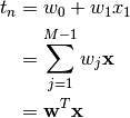
   pdf("snakes-hist.pdf",height=6,width=6)
   hist(y,col='grey',main="distribution of y")
   dev.off()
   

   \begin{figure}
   \begin{center}
   \includegraphics[ext=.pdf,scale = 0.9]{"snakes-hist"}
   \end{center}
   \caption{This is the figure caption}
   \end{figure}
   

4. Add an example of a formula. After all it is .

   

   Here are the commands you will need:

   • \usepackage{amsmath}

   • subscript x_{i} superscript x^{i}

   • \sum^{}_{}

   • \mathbf{}

   • \begin{align}
        x^{2}      &= x \times x \\
        e^{\ln(2)} &= 2
     \end{align}
     

   Note

   what if you use align*? or if you put the & at the beginning of each line?

6. Show and example of how to save data to file. The following code will help you figure it out

   a <- rnorm(10)
   b <- rnorm(10)
   ab <- data.frame(a,b)
   dump("ab",file="ab.R")
   rm(ab)
   source(file="ab.R")
   ab
   

7. Edit/create your model, inits and command files

   First try this with the provided files. Then if you wish the model and command files can be written to file from your sweave documents using the cat and sink commands. The inits file can be written with dump.

   cat("model{
       # priors
       mu ~ dunif(0,5000)             # populaiton mean
       sigma ~ dunif(0,100)           # populaiton sd
       tau <- 1 / sigma * sigma       # Precision = 1 / variance
   
       # likelihood
       for(i in 1:N){
           mass[i] ~ dnorm(mu,tau)
           }
       }
   ",fill=TRUE,file="model-of-the-mean.txt")
   

   # bundle data
   jagsData <- list(mass=mass,N=length(mass))
   
   # inits function
   inits <- function(){list(mu=rnorm(1,600),
                       sigma=runif(1,1,30))}
   
   # Parameters to estimate
   params <- c("mu","sigma")
   
   # parameters for MCMC sampling
   nc <- 3       # Number of Chains
   ni <- 5000    # Number of draws from posterior (for each chain)
   nb <- 200     # Number of draws to discard as burn in
   nt <- 2       # Thinning rate
   

8. run it

   library(R2jags)
   jagsfit <- jags(jagsData,inits=inits,parameters.to.save=params,
                   model.file="model-of-the-mean.txt",n.thin=nt,
                   n.chains=nc,n.burnin=nb,n.iter=ni)
   

   Not using R or R2jags?

   The alternative procedures is:

   • save the model file
   • save the data in a file
   • create inits files
   • create a command file that specifies file names and MCMC parameters
   • make the plots by parsing the results files (CODA)

   ~$ jags line-reg-simple.cmd
   

   or

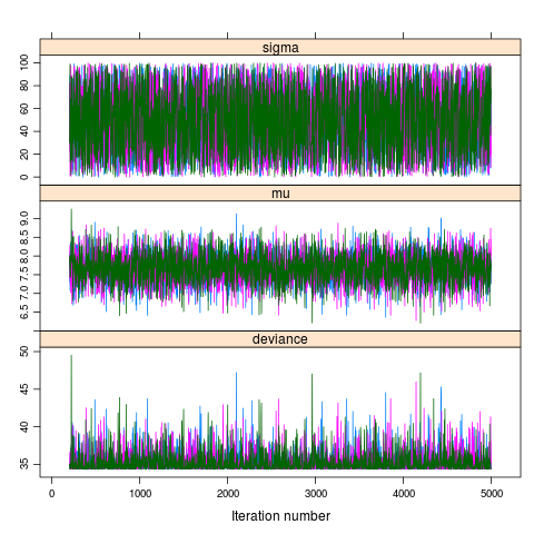
   system("jags line-reg-simple.cmd")
   

9. Plot the chains (posterior)

   jagsfit.mcmc <- as.mcmc(jagsfit)
   pdf("model-of-the-mean-chains.pdf")
   xyplot(jagsfit.mcmc)
   dev.off()
   pdf("model-of-the-mean-densities.pdf")
   densityplot(jagsfit.mcmc)
   dev.off()
   

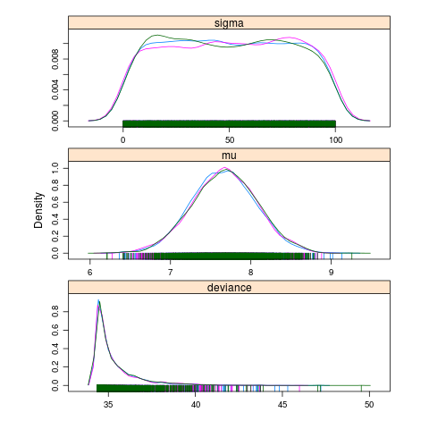
DIC is an estimate of expected predictive error (lower deviance is better).

Download the R script: ModelOfTheMean.R